(Continued from the previous post).

Having thus established that an extra temperature transmitter for the headspace leads to useful possibilities, we now move in the direction of developing the mathematical equation with instantaneous IV on the LHS. The fulcrum of such a development is the density of the reaction mixture which eventually leads to quantification of the headspace gas. This is actually a breakthrough allowing a lot more reliable accounting of hydrogen gas flowing past the external transmitter paving the way for estimating the IV-lowering hydrogen. Of course, the density of the reaction mixture has other uses also – mainly mainstreaming of hydrogention kinetics by helping replace I with [db], mols/lit.

Devlopement of relevant mathematical equations:

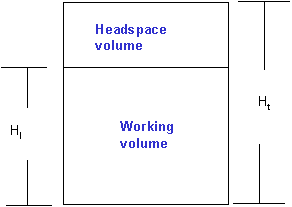Headspace volume (V_hs): V_hs = V_re – V_rm which are instantaneous reactor and reaction mixture volumes during a specified hydrogenation cycle on a stilled reactor ie with hydrogen bubbling and agitation stopped.

V_hs = V_re – M_rm/ρ, where M_rm is the mass of reaction mixture (charge + added catalyst + m₁) and ρ, the density at that stage. Read the ‘note on reaction mixture density’ later in this post.

V_hs = V_re – (1000x + 10xy + m₁)/ρ where x is the charge size in MT and y, the % addition of the catalyst with known activity and Ni content. m₁ is the cumulative chemical hydrogen consumption in kgs.

V_hs = V_re – (1000x  + 10xy +m₁)/ ρ

Note: 1. While a protocol to determine V_re as a function of T, can be developed, it is best sourced from the supplier.

2. The query that m₁ is being used here on the way to determining m₁ is genuine. In reality m1 is such a small fraction of the total mass that it can be ignored. Accounting for absorbed hydrogen is also possible by noting that a plant set up easily knows the relationship between m₁ and m form past practical experience e.g. m1/m can be called a factor ‘f’ and m₁ in the above equation, replaced with fm.

 Headspace gas quantity, m_hs:

pV_hs = nRT_hs, hence, n = pV_hs/RT_hs, thus, m_hs  = 2 pV_hs/RT_hs

At any stage of a specified hydrogenation cycle, let

m = cumulative hydrogen past the flow transmitter

m₁ = chemical (IV lowering) consumption

m₂ = hydrogen vented/evacuated so far at the conditions at each venting and a large fraction of the then V_hs. To avoid complexity, we will not detail that mathematics which is close to the p-T-V application.

m₁ = m – m₂ – m_hs where m_hs is the residual hydrogen at the end of the cycle.

If x is in MT, and m₁ in kgs, this is equivalent to absorption of 127m₁ kg iodine in 1000x kg oil for given ∆I.

That ∆I = 12.7m₁/x = (12.7/x)(m – m₂ – m_hs)

Therefore, I = Io – (12.7/x)(m – m₂ – m_hs)

Note: (i) This equation obviously obviates the in-line IV measurement. The requisite mathematical equation to determine ρ is derived below, the determining protocol will follow later.

(ii). ρ also helps determine [db], mols/lit : [db] = 0.0394 ρI.

(iii). Today’s all-weld reactor designs leave the mechanical seals at the exit of the agitator shaft, the stem seals of all the valves above the reaction mixture free surface and the gaskets to reactor mountings and fixtures as the potential leakage points. The volume of hydrogen leaked, V_lk, is expected to be (and must be, for safety) small enough to introduce negligible error when not considered. A special note (probably an entire post) will be incorporated somewhere to explain its importance and its determination as a ‘constant’ for each reactor to be periodically validated.

(iv) Smart operators can discover the relationship between m₂ and m_hs and simplify further. If (m –m₂ – m_hs)/m is assigned factor ‘f’, ∆I = I_o – 12.7mf₁/x. Since x is always known, I can be calculated without the back of an envelope. Interestingly, m₂ happens at lower T and is not complete removal of all V_hs gas; m_hs is total V_hs gas at higher T.

(v) Variation in ρ because of drift towards tdb formation caused by catalyst poisoning are expected to be too small to notice easily.

Adaptation I: Extra pressure transmitter on the side of the reactor

The mathematical equation: On a stilled reactor with hydrogenation halted, at any intermediate I, if

p’ = pressure at a spot above the bottom dish-cylindrical portion joint

h = depth of that spot from the free liquid surface

p_hs = headspace pressure

ρ = density of the reaction mixture

g = gravitational acceleration at that location

(p’ – p_hs) = hρg

ρ = (p’ – p_hs)/hg

Adaptation III: Leveraging hydrogenation thermochemistry

The inviolable relationship between the heat evolved as result of a  chemical reaction and its extent is a juicy opportunity to, prima facie, track the progress of the reaction by measuring the heat evoplved up to any stage. When it is done for a short duration ∆t, it indicates the average of the rate of the reaction (dI/dt and d[cis to trans]/dt) during that time span. (Though I have thought it up, it can’t be new to hardcore chemical engineers.) The issue is then reduced to measuring such heat evolved by deploying the specific heat of the reaction mixture, M_rm and the observed ∆T.  This adaptation is simply conversion of the reactor into a calorimeter by arranging to measure the heat transferred to cooling water by a known mass of the reaction mixture, leading to measured ∆T. Let’s call this version of exploiting heat-reaction extent relationships, thermostoichiometry.

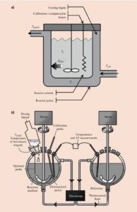(The inviolability of the Heat of every reaction, ∆H_r, stems from the fundamental fact of unique, fixed enthalpies of each bond that makes up every molecule participating in the reaction. Standard heats of hundreds of reactions are available in literature and the use of those requires the approximation of their applicability at other – usually higher – temperatures. Here we will be developing the modalities of knowing the continuous variation of the specific heat of the reaction mixture through out the reaction cycle. Its multifaceted utility is the subject of another post.)

The following sequence of steps simplifies the understanding of the ‘scheme’ and, more importantly, the ideation behind it:

Steps for measurement of the dynamic ‘s’ of the reaction mixture

For lucidity, we focus on a standard hydrogenation protocol starting at 120 deg C, rising to 180 deg C and remaining constant till the end.

1. Addition of a mass flow meter in the external cooling water lines and a temperature transmitter each in the inlet and the outlet turns the reactor into a calorimeter.
2. In this avatar, it can measure the heat transferred to the cooling water by the insulation, the reactor metal and the reaction mixture, per se’ during a small ∆T, say, 151 to 149 deg C at IV ‘I’. The reaction would have to be stalled from its onward journey temperorily and after the measurement, the reaction can resume.
3. Subtracting the calculated heat lost by the reactor metal and the insulation, the heat transferred from the reaction mixture is obtained.
4. Since ∆T and M_rm are known, the specific heat (s = Q/(M_rm*∆T) at IV ‘I’ and temperature T (say, 150 deg C) of the reaction mixture identified uniquely from the known protocol is known. This is repeat use info, to be reverified at the processor’s discretion.
5. Repeating the same protocol at diffetern temperatures during the rising temperature stage, (say, at 120, 130, 140, 150, 160, 170 and 180 deg C) for a soybean protocol, we get 7 values of ‘s’ at these increasing temperatures, ∆I’s and corresponding reaction mixture compositions.
6. During the terminal constant temperature stage, the temperature remains constant and the dynamic heat of the reaction gets measured cumulatively. At close to expected m₁ for the cycle, the reaction can be stopped and exactly the same protocol followed as the one at the start of the isothermal stage.This time it will reveal ‘s’ of the terminal reaction mixture at 179 deg C because of which it will be close to ‘s’ at the start of the isothermal stage because the ‘s’-changing composition change is nominal and the physical reason for the change is absent.
7. Important: The selected T-based milestones automatically select somewhat unevenly distributed corresponding ∆I (or I) and take cognizance of the stronger variation of ‘s’ with T.  The plot of s vs T is thus automatically the plot of s vs ∆I. Essentially, therefore, ‘s’ is known continuously through out a cycle, making it possible to track the heat evolution (Q). This will be developed further later.

Note: 1. The detailed protocol can be seriously elaborate because of the precautions to be taken for accounting of quantity of water in the circuit. 2. The cooling at every interruption needs to be slow enough to allow ‘steady state heat transfer’ so that the temperatures of the insulation and the reactor metal are reliable for heat transfer calculation. 3. Similarly, precautions must be taken to ensure ‘single phase water flow’ at the outlet of the cooling circuit so that the registered temperature reflects the actual heat content. 4. Obviously, the ‘2 deg C’ band for cooling is arbitrary and small to usefully reflect ‘s’ at the mean temperature. In reality any accurately measured ∆T close to 2 deg C is okay.

A note on ‘reaction mixture density’

Literature is replete with the data on density/specific gravity of pure chemicals and known standard materials like soybean oil (at specific temperatures) and its variation with temperature. However following issues emerge when we try to deploy their numerical values in mathematical equations leading to insights like [db], mols/lit = 0.0394ρI or V_rm = M_rm/ρ.

1. They obviously don’t apply to ‘reaction mixtures’ of which they are components.
2. In case of edible oils, specification of ‘raw’ or ‘refined’ is sometimes disconcertingly, missing probably alluding to the the closeness of the values in either case. Interestingly, the input oil to hydrogenation is almost invariably degummed/neutralized and bleached oil which is strictly neither raw nor refined. Of course, this nitpicking would have been redundant, if othert serious objections to readymade data for standard materials did not exist.
3. When hydrogen bubbling has been stopped, the bubbles must immediately buoy up into the headspace and dissolved hydrogen must spontaneously diffuse into the catalyst pores and disappear thru consumption. (Calculations of mols/grams of hydrogen in the rm at any instant and the time required for them to disappear thru reactive consumption at various ∆I in a protocol is an interesting challenge; this author has been a bit disconcerted by the seeming absence of the solubility data as a function of T and p.) Thus after the ‘stilling’ of the reactor, it contains in the ensuing minute or so, a still practically homogeneous near-colloidal mixture of oil and the catalyst. Given the chemical changes that hydrogenation has caused, the even the filtered oil at that stage is a unique material in itself. Interestingly, its chemical identity for a given hydrogenation protocol, is unlikely to differ much across batches unless the catalyst poisoning signals have been grossly ignored – a highly unlikely possibility in todays demanding time.

Thus the pressure sensed at a specific depth in the still reaction mixture is a good reflection of its density and nothing else can take its place.

4. The foregoing discussion applies to isothermal, isobaric ‘experimental’ hydrogenation; it cannot be ‘real life’ given that it needlessly abandons the utility of ‘p’ and ‘T’ in guiding the reaction trajectory. The real life, commercial hydrogenation typically goes thru the rising and constant temperature stages during which the actual rate equation is: d[db]/dt = A.exp(∆E_a/RT).[db][hyd], accepting the first order vis-a-vis both reactants (2^nd overall). Here, the temperature factor additionally complicates the density for a major part of the cycle which further bolsters the argument for the discovery of the density of the reactuion mixture during the entire course of hydrogenation cycle continuously.

Getting saturated with my obsession with ‘hydrogenation’? We will emerge from this shroud soon to talk about the history of food processing and the teachings from it that we have missed.

Next Post:

Adapting the Industrial Reactor for Research – III

ρ in instrumentless tracking of IV and other applications

Visit Disclaimer