Relevant equations:

V_hs = V_re – (1000x + 10xy + m₁/ρ

m_hs = 2pV_hs/RT_hs

 I_o – (12.7/x)(m – m₂ – m_hs)

A close look at V_re, V_rm and V_hs :

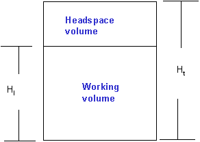The reactor volume (V_re) distribution as we move up the reactor from the lowermost point in the bottom dish is erratic and cannot be calculated easily thru geometry. It further changes with the temperature. Thankfully, we don’t need it because we are not calibrating the reactor. Interestingly, it can be done easily ‘empiricaly’ simply by filling up the reactor to the brim (till water begins to come out from the mechanical seal aperture) and then simply go on draining gradually it into a tank mounted on load cells and noting the height of the water mass. Equally, the reactor can be mounted on load cells. Note that this works with water only at close to room temperature.

V_re as a whole varies with temperature and the graphical representation of this variation is quite easy but we will not digress and trust the reactor supplier to provide it.

V_rm is essentially V_re up to the free surface of the reaction mixture. ‘V_rm as M_rm/ρ’ (all three instantaneous) is fundamental and since M_rm (original oil charge + the catalyst added + m₁ up to that instant) and ρ are known continuously V_rm is also similarly known. The apparent distortion because of agitation and bubbling is redundant because the liquid is incompressible. Interestingly, ρ vs I, t, T, m₁ plots are practically constant across identical batches and hence a long term asset for a given protocol. Its utility as a reaction-accentricity indicator (catalyst poisoning and unplanned hydrogenation/isomerization rate ratios) is limited because of the expected and essential low variation in it.

V_hs as the difference, is obvious, and has its own variations. Combined with the acceptable ideal behaviour of hydrogen in the headspace conditions and the newly introduced T_hs measurement, m_hs can be easily known from the Universal Gas Law. This immediately leads to m₂ – the gas vented/evacuated in the initial stages and m_hs – the residual, unreacted headspace gas at the end. We will leave these interesting calculations to STEM students.

Since it has to be large enough to prevent escape of entrained oil along with vented or evacuated hydrogen, the reactor top has to be far enough from the ‘boiling’ gas/liquid interface. The headspace always occupies the top dish completely and extends into the upper cylindrical portion of the reactor. In more intricately designed reactors, headspace is used more elaborately. Additionally, there are mancovers, glass window fittings, instrumentation, pipe attachments, valves etc.

The subtle nuances of ‘m₁’ – the IV-lowering hydrogen:

The leakage losses: Obviously, Chemical (or IV lowering) hydrogen consumption = (hydrogen past the external flow transmitter) – (hydrogen evacuated/vented at respective headspace p, T conditions) – (residual headspace hydrogen at the end of the reaction cycle, again at the then existing p, T conditions.) If the leakage losses are determined (we will see if we can devote a separate post to it), the equation becomes even more conservation-compliant.

In today’s predominantly all-weld reactor designs, the agitator shaft seal at the top and all types of gasketed joints and valve stem seals are the only leakage spots for hydrogen. For every specific hydrogenation protocol, the leakage cannot vary noticeably because of the practically constant cycle length, commonness of the reactor features and, most of all, the sanctity of the meticulously determined reaction conditions, especially p,T.  Obviously, these would be losses beginning with the external flow transnmitter (i.e. ‘hydrogen issued for hydrogenation’) up to the reactor and the end of every reaction cycle.

How exactly does m₂ – the headspace hydrogen quantity – help?

1. It helps determine vent/evacuation hydrogen (m₂) in the same way as residual ‘static’ hydrogen (m_hs) at the end.
2. This helps fairly accurate mass balance and hence fairly accurate determination of the all-important m₁ that can be connected with ∆I and hence I. It also helps explain why the flow transmitter-based estimations of I are misleading. Presumably, the success in connecting ‘m’ of successive identical batches with analytically found I (even with slippages) bypassed the need to monitor intermediate ‘I’ during hydrogenation, which remained dispensable. This is why literature quotes marginally higher than stoichiometric ‘hydrogen requirement per MT oil per IV drop’.
3. The leakage losses are more accurate with m₂; tracking them is important for safety and process costing.

A brief review of the density change during hydrogenation:

As we already know, the density is expected to decrease gradually and continuously (in a characteristic and not necessarily linear way) during rising temperature stage of commercial hydrogenation – because of (i) reducing unsaturation (ii) increasing TFA and (iii) rise in temperature. Most of the partial hydrogenation (∆I < I_o, usually a fraction of I_o) happens during this stage which makes the isothermal duration limited after cooling is applied at the selected maximum temperature. (A point to ponder: the selection of this maximum temperature determines how the total hydrogenation time breaks into rising T and isothermal stages. This is more intricate than may prima facie appear and leads eventually to the realization that p, T (and, for that matter, all the factors) should be smartly manipulated to optimize reaction rate with quality.

During isothermal hydrogenation (which is, in any case, usually a small fraction of planned ∆I), the purely chemical density change is expected to be nominal with the ρ vs. t or ∆I curve stooping only slightly and breaking away from the rising temperature stage with a smaller slope. We have already found that the density of the reaction mixture must be discovered as off-the-shelf data may not inspire confidence.

Tracking I continuously during hydrogenation:

It is obvious that (i) This obviously happens thru equation 5 above. The protocol has been briefly described below. (ii) This obviates the in-line instrument. (iii) This technique is based on hydrogen accounting which also has other benefits.

In my happily trans-ignorant days which also happened to be resource-strapped, our guide for judgement of ‘extent of the reaction’ during hydrogenation was the melting point of the sample drawn from an interrupted batch, tested right next to the reactor. Note that the nudge came from the gross gas consumed. Sending the sample to the lab far away for IV determination and keeping the reaction in limbo until it was impractical. Being compelled to spruce up your game is one of the less visible effects of competition. Obviously, the long cycles were the result of flawed pre-hydrogenation processing and reactor design.

When the refining turned continuous, there was perceptible rate increase and reduction in catalyst consumption. Today’s young engineers used to watching PLC panels would take time to comprehend that oil could be refined in a batch neutralizer. Far from being embarrassed about my ‘rudimentary upbringing’, I am extremely proud of having produced acceptable refined oils and vanaspati in a batch process.

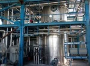(In 1985 – or was it 1986 – NDDB received India’s first lot of canola oil from Canada under a Cooperative Union of Canada grant and refining it fell on my young shoulders. Nobody had a clue on the ‘recommended practice’ and my vanaspati production was occupied with the newly installed continuous degumming-cum-refining plant. In an ‘occupied state’, I began refining canola oil in the batch plant. Soon the batch bleachers were released for filtration. I still shudder at the near total failure of the earth-carbon laden oil to filter. It was as if the filtercloths were getting wax coated with the first flush of the bleached oil slurry. I have rarely felt more inadequate in my life. That night, as I left the plant for a meal with my newly minted wife, I knew that I would be returning soon.

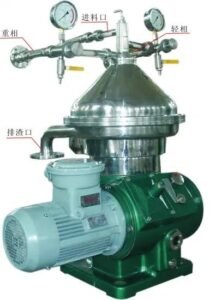I walked to the plant from home after midnight and, on the way, decided that all the oil under process should receive a centrifugal ‘clean up’ and directed the requisite arrangement – an ungainly  combination of rigid and flexible piping –  through out the night before reaching home at day break. When I again reached the plant after a 2 hr nap, the first lot of centrifugally cleaned oil was being released for bleacher filtration. Imagine my delight when the filterpress channel started overflowing immediately! Figure out what happened. See? ‘Cases’ are not the monopoly of M Schools!)

Resuming:  operators decided to offer the sample for MP measurement on the basis of how a blade of solidified reaction mixture slipped off from an ice block, melted on the back of their palm. And, if it could be kneaded in the palm (which happened often with palm oil). That nudged the formal capillary slip mp measurement.

Quickly pivoting from nostalgia, tracking the decreasing I – the more useful indicator of the reaction progress is simply:

Instantaneous IV, I = I_o – 12.7m₁/x

where m₁ is the chemical hydrogen consumption in kgs, ‘x’ is the charge size in MT. The kinetically compliant [db], mols/lit follows from [db] = 0.0394ρI, where ρ is the density of the reaction mixture because of addition of m₁ grams of hydrogen in the oil which had original IV of I_o.  Incidentally, it can be shown that:

[db], mols/lit = 0.0394ρI_o – 0.5m1ρ/x……………………………6

where x is in MT, m₁ in kgs and ρ is in kgs/lit. Note: 1. The sneaking in of ρ the moment ‘concentration’ comes in. 2. This equation is essentially [db] = [db]_o – ∆[db].

Note: 1. For a specific hydrogenation cycle in identical reactors, the reaction trajectories are practically the same.  In fact, this is a precondition to make a certain tonnage of a hydrogenated ‘stock’ with known functionalities and hence application, e.g. as bakery shortening or frying oil. This stems from comparable extents of IV change and TFA formation (or dI/dt and d[tdb]/dt for the duration) essentially resulting in closely comparable final product composition.

2. The utility of this accurate accounting of hydrogen is maximum in the initial stages when mhs is a larger fractions of m and leakages are negligible. Obviously, the gap between m and m₁ is maximum then and hence the relationship between m and ∆I is tenuous. Thus this technique is a blessing in, say, brush hydrogenation of soybean oil and locating the CLA maxima described later which obviously banks on stopping hydrogenation near the linoleic acid maxima.
3. This is made possible thru accounting that inculcates a spirit of ‘cost consciousness’; in today’s competitive times, the gap between hydrogen paid for and hydrogen that added realizable economic value, must be kept at the minimum.
4. This also minimizes the explosive risk by pointing out leakages which can be invisible and inaudible.
5. This technique obviously requires determination of dynamic ρ which has other uses as described below.

A brief outline of the protocol

The following transmitters/software send their designated signals to a programmed microprocessor (eq. 3):

The head space pressure transmitter…..p_hs

The reaction mixture pressure transmitter …..p

The RF position transmitter ………………….h

The density indicating signal as well as plot…………. ρ and ρ vs t, T, m₁, I.

V_re………………………………………..from the memory

V_rm …………………..from M_re/ ρ

V_hs……………………………from the difference

m_hs……………………………instantaneous as well as vs I.

m₁ from the requisite equation.

I from the applicable equation.

Other derived utilities of ρ:

1. Continuous [db], given that [db] = 0.0394ρI. The [db] vs t curves would be classical kinetic curves that would yield d[db]/dt vs t as well as [db] curves. As any chemical engineer knows, these curves are loaded with possibilities. ln[db] vs t curves at various constant p,T (reaction kinetic isotherms; note that the [hyd] factor is taken out by constant p,T) are another great research avenue. Literature reports some such IV-based cottonseed oil hydrogenation isotherms that curve towards the log(I) axis at lower temparatures and increasingly curve away as T increases, ironically producing a straight line (!) at a particular temperature befor beginning to curve away from the ln(I ) axis. Obviously, the straight line is a ‘coincidence’ that does not yield ‘k’ at that temperature – exploring the reason behind that linearity would be the stuff of a bright chemical engineer’s dreams.
2. A one time [cdb] vs t curve for a specific commercial can be created from periodic sampling for full hydrogenation (∆I = I_o), e.g. at IV 130, 110, 90, 70, 50, 30 and 0 for soybean oil. When superimposed on a computer generated [db] v/s t curve for that hydrogenation cycle, a [tdb] vs t curve can be derived from this which is bound to have a maxima, with one end at (0,0) and the other at (‘t’,0) where ‘t’ is the cycle length for full hydrogenation. This curve can be exploited smartly.
3. [db] vs t is classical even if db per se’ is not the classical reactant. But similar curves from the literature for hydrogenarion of, say, cis, triolein or even cis oleic acid and comparision with an oil hydrogenation [db] vs t can be highly educative.

Next Post:

Adapting the Industrial Reactor for  Research – IV

Leveraging thermochemistry for useful reaction insights

 

Visit Disclaimer