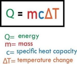The estimation of the heat that a known quantity of substance must have absorbed to have an observed ∆T is essentially heat quantification from ∆T, s and m numbers. This simple realization is a strong nudge to try to measure a reaction exotherm in a bulk batch reaction, essentially thru determination of the specific heat ‘s’ (or heat capacity as an extensive property) of the reaction mixture. In this case, we have already noted that ‘s’ is challenging given its unknown variability with the composition and temperature. This is pronounced in most initial cases of commercial hydrogenation accounting for most of ∆T and ∆I-led composition change.  As a corollary, know ‘s’ through out your ∆I and you know the cumulative heat release Q for a largish ∆T and dQ/dt at any stage.

Leveraging this to generate fresh data and process it to derive insights in reaction quality and extents is the essence of the next few posts. Breaking down ‘reaction extents’ into moles (and hence kgs) of reactants consumed or specific products formed and hence create techniques like reaction tracking or locating specific yield stages of a given product is stoichiometry. When such a product is TFA or, on a positive note, CLA, it suddenly starts looking interesting. A combination of the two is thermostoichiometry.

There are two major reaction extents in partial hydrogenation, each with its own heat evolution and impact on quality. Discovered Q, therefore, must be apportioned to be meaningful. At the end of the tunnel to process this apportionment is the reward: the extents of saturation of double bonds (∆I) and of isomerization of cdb to trans. Enticing, no? Especially if this can be done during live commercial hydrogenation, without reaction interruptions and sample withdrawals and at at a low cost? Oh, I know, I know, hydrogenation of oils for food uses is almost dead, so why this fuss? An invisible hand, maybe.

Equations connecting heat release and reaction extents

The following equations, during hydrogenation, are self-evident

1. [db] = [cdb] + [tdb]. Initial [tdb] = 0 in plant source oils.
2. No. of moles of cis and trans double bonds in the reaction mixture at any intermediate stage = [cdb](M_rm/ρ) and [tdb]( M_rm/ρ). And the sum corresponds to I (= I_o – ∆I).
3. d[db]/dt = d[cdb]/dt + d[tdb]/dt. These ‘rates’ can be parts of interesting kinetic equations – an avenue for further research. Note: ‘n moles’ is stoichiometry, [db], moles/lit is kinetics and ∆H kcals/mole is thermochemistry – components of thermostoichiometry.

Now, the cumulative exotherm of a given extent of hydrogenation in a commercial batch (or ∆I of a specific cycle) = Q = ∆H of direct saturation of n1 moles of cis double bonds + ∆H of  isomerization of n₂ moles of cis double bonds to trans + ∆H of hydrogenation of n₃ moles of trans double bonds*.

(* Comes into play after the [tdb] maxima when the [tdb] vs t curve has inverted and the slope or d[tdb]/dt has a negative value implying net tdb hydrogenation. Before that, any hydrogenation of tdb is the second step of cdb hydrogenation and hence is accounted for as a part of cdb hydrogenation in parallel to their direct hydrogenation. Note: tdb hydrogenation ∆E_a is higher than for cdb. [db] vs t plots in literature show a precipipitous fall in the initial stages (especially in case of soybean oil) because of high cdb hydrogenation and isomerization rates fuelled by high [cdb] and low ∆E_a of isomerization, dampened only by the usually relatively low initial Trm.

Thus, initially, (rate of tdb hydrogenation) < (rate of tdb formation thru cdb isomerization) and d[tdb]/dt > 0 with reducing curve slope towards the maxima.

 At the [tdb] maxima, (rate of tdb hydrogenation) = (rate of tdb formation) and d[tdb]/dt = 0.

Thereafter, (rate of tdb hydrogenation) > (rate of tdb formation); d[tdb]/dt < 0 with a long drawn out flattish-curved taper towards time or ∆I axis – in total contrast to premaxima pattern. This is obvious from fast decreasing [tdb] and high ∆E_a. Keen observation of the experimental hydrogenation curves in the literature, especially of soybean oil at high T,p does indicate a steep initial dI/dt and a long drawn out reduction in the slope of the curve towards completion, especially for full hydrogenation.

Note that isomerization of cdb and hydrogenation of tdb are the single steps that lend themselves to kinetic analysis with ‘pure’ ‘k’ values in the Arrhenius eaquation. As already discussed in detail earlier, ‘A’ is questionable even in these cases.

Checking out the ‘steady state’ of heat traqnsfer

Heat released as a result of the reactions is absorbed by the reaction mixture, and by further heat transfer, to the reactor and outward into insulation – three ‘resistances’ in series – two if you treat the reaction mixture as the ‘source’ of heat. The reactor metal obviously has high thermal conductivity and hence nominal temperature gradient across its small thickness. Insulation, to be effective enough, has to have low conductivity and ample thickness which means a steep gradient and more path length combining to ensure barely measurable temperature difference between the outer skin and the atmosphere.

In essence, the heat content rise of the trio of the reaction mixture, the reactor and the insulation can be reasonably equated with the heat released as a result of the extent of the reactions up to the stage of measurement. Given that the insulation open skin temperature is easily measurable, more accuracy thru more complete accounting can be obtained by the data available on heat loss per sq. m., per hour per on exposed surfaces, especially in cold, windy conditions. Hope America and Europe design their plant layouts to exploit the heat convected/radiated by hydrogenation reactor insulations to lower the internal heating costs. Air-cooled hydrogenated stocks before filtration? 

Practical observations put hydrogenation heat evolution at 940 to 945 kcals/MT/IV; that this is less than the heat of hydrogenation of ethylene to ethane is interesting.This puts the average heat release rate for a 4hr reduction of IV of 20 MT of soybean oil from 130 to 70 @ about 4700 kcals/min.This would raise the temperature of the charge @ about 0.43 deg/min @ sp ht of about 0.55 kcal/kg/deg C approx avg  sp. ht.

Note: Given the rising temperature and isothermal stages of typical commercial hydrogenation, the rate-raising influence of the temperature on the rates – the energetics factor – is superimposed on the rate-decreasing concentration factor. I have yet to come across an I or ∆I or m₁ or T vs time curve for commercial hydrogenation – obviously my limitation. For the version of hydrogenation (earlier mentioned as a potentially smart technology optimizing rate and selectivity) each ‘reaction thermogram’ would reflect a specific variable management protocol including temperature. However, the steady state presumption cannot work in case of ‘modern, superfast’ hydrogenation, incidentally exposing the reactor and the insulation to thermal stress.

Generation, transmission and absorption of heat in the reactor

Imagination helps ‘see’ a phenomenon from different angles and a selected ‘angle’ can be rewarding if nudged by purpose. e.g…..

1. Chyavanprash as a spiced up, ghee-enhanced gooseberry jam.

[The poor value proposition of conventional jam (and mfg costing sustained mainly by the possibility of ‘fruits fit for jams’) and smartness of chyavanprash with fat-improved bioavailability are an interesting contrast. Incidentally, chyavanprash needs the ghee given the additional presence of spices and herbs with potentially low polarity fat solubles. West can ask us for a ‘western’ version that they will lap up both for a familiar, enticing taste and real benefits.]

2. A batch reactor as a calorimeter.
3. Domestic pressure cooker as a sterilizing autoclave.
4. Milk powder and condensed milk as Indian ‘khoya’ makers.
5. Heart as a positive displacement diaphragm pump. The bicuspid, tricuspid, pulmonary and aortic valves as NRV’s. Blood vessel network as heart’s plumbing with organs as ‘resistances’ to flow; the glomeruler distortionss adding extra resistance in kidneys leading to raised bp.

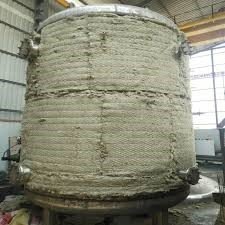Similarly, a batch reactor hosting an exothermic reaction can be modelled as a source of heat rising from its chemically transforming contents. This heat, is first absorbed by the heat producing mass itself and the remainder spreads outwards crossing two ‘resistances in series’ before the necessarily meagre remainder merges with the surroundings. These resistances are the highly conductive reactor metal and highly resistive insulation between the metal and, nominally, the surroundings. Applications of a few justifiable approximations (see below) allow fairly reliable estimation of the heat absorbed by the three classes of materials and hence of the exotherm per se’.

Now consider a hydrogenation spell (∆I) leading to cumulative release of heat of saturation and isomerization (Q) heating up the reaction mixture, the reactor and the insulation or water during the isothermal stage.

(i) Heat absorbed by the reaction mixture is (1000x + 10xy + m₁).s.∆Trm where m₁ is the chemically added hydrogen up to that stage. (Ref post no. 47 : Adapting the industrial reactor for research, Further deep dives in adaptations).  Note: here m1 increases continuously, ∆Trm increases according to planned process protocol and s varies as defined by the discovered s vs (t, ∆I, T) plot. A code needs to be written for calculation of (1000x + 10xy + m₁).s.∆Trm continuously till the reaction closure and emergence of the integrated number. This applies to similar terms below also.

(ii) Heat absorbed by the reactor metaI: Ignoring the temperature drop across its highly conductive thickness of the order of 20 mm and accepting the reaction mixture/reactor inside skin interface as Trm because of high turbulence and practically non-exixtant static film, this is (mass of reactor metal)(∆T_rm)(Sp. ht. of reactor metal) or M_re.s_re.∆T_rm.

(iii) Heat absorbed by the insulation: Taking outer skin temp as Tamb and a linear temperature gradient across its thickness, avg temperature of the insulation material = (T_rm + T_amb)/2. Hence heat absorbed = M_ins.s_ins.∆T_rm/2. In both cases 2 and 3, s variation with T has to be available. Note: The application of insulation must necessarily ensure that it is isotropic when in use. For the more meticulous, the avenue of using the heat lost to ambience per minute per sq. m. and hence the insulation as a whole, from empirical equations in the literature exists. The outer skin temperature is obviously measurable and the heat losing area is known.

In the next two posts, post will wrap up the applications of thermostoichiometry of hydrogenation and rounding up topics and then re-emerge in the world of foods, their processing and their impact on our lives.

Next Post:

Adapting the industrial reactor for research – V

Quantification and apportionment of reaction heat and its rewards

 

Visit Disclaimer